Go Top

Go Top

Definition & Properties 

Diff. Eq., Transfer Function & DTFT

Sinusoid Explanation

Magnitude & Phase Response

Poles, Zeros & Filter’s Shape

Homework:

p274: 7.1,   p275: 7.5,   p278: 7.20

Frequency Response频率响应

   The discrete time Fourier transform (DTFT) of

        System Impulse Response.

F{ h[n] } = H (Ω),
F-1{H (Ω) } = h[n],

Properties

       Given H(Ω) of h[n]:

        P1. Periodicity

             H(Ω) = H(Ω+2π)

        P2. Time Delay

             F{ h[n-M] } = exp(-jMΩ) H (Ω)

        P3. Frequency Shift #

             F{ exp(-jΩ₀n) h[n] } =  H (Ω + Ω₀)

        P4. Linearity

        F{ a h₁[n] + b h₂[n] } = aH₁ (Ω) + b H₂ (Ω)

        where  H₁(Ω)=F{h₁[n] }, H₂(Ω)=F{ h₂[n] }

        P5. Conjugacy  #

             F{ h^* [n] } = H^* (-Ω)

              When h[n] is real, H^* (-Ω) = H (Ω)

        P6. Difference

            F{ h[n] - h[n-1] } = [1-exp(-jΩ)] H (Ω)

        P7. Flipping  #

             F{ h[-n] } = H (-Ω)

        P8. Upsampling  #

             F{ h[n/k] } = H (kΩ)

        P9. Differential  #

F{ n h[n] } =

        P10. Convolution   #

           F{ x[n] * h[n] } = X(Ω) H(Ω)

           where  F{ h[n] } = H(Ω) , F{ x[n] } = X(Ω)

        P11. Product   #

F{ h1[n] h2[n] } =

           where  F{ h₁[n] } = H₁(Ω) , F{ h₂[n] } = H₂(Ω)

        P12. Parseval  Theorem:   #

             |H (Ω)|²  : Power Spectrum Density

Difference Equation,

Transfer Function & DTFT

   Difference Equation of ARMA Model

   自回归滑动平均模型的差分方程

                 a₀y[n] + a₁y[n-1] + L + a_Ny[n-N]

              = b₀x[n] + b₁x[n-1] + L + b_Mx[n-M]

   After DTFT using P2,

                 Y(Ω) [a₀ + a₁e^-jΩ + L + a_Ne^-jNΩ ]

              = X(Ω) [b₀ + b₁e^-jΩ + L + b_Me^-jMΩ ]

   So,

              H(Ω) = Y(Ω) / X(Ω)

   Transfer Function

                        z    =>    exp(jΩ)

Sinusoid Explanation 

       When  the input x[n] is sinusoidal,

            x[n] = A cos(nΩ₀ +Φ_x)

       Short form notation of DTFT

            X(Ω₀) = A Ð Φ_x   ,  H(Ω₀) = G Ð Φ

       According to

            Y(Ω) = X(Ω)H(Ω)

       We have

            Y(Ω₀) = X(Ω₀)H(Ω₀) = AG Ð (Φ_x+Φ)

       Thus

                  y[n] = AG cos(nΩ₀ +Φ_x+Φ)

       Frequency Response is a collection

        Magnitude Gain & Phase Delay

        for all the frequencies.

                    H(Ω) = G(Ω) Ð Φ(Ω)

 

 

 

 

 

 

 

 

 

 

 

 

 

 

 

 

 

 

 

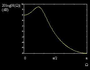
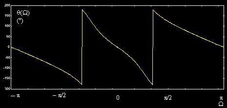
Magnitude  & Phase Response

     The Shape of the filter is the shape of the

     Magnitude Response.

     Rewrite H(Ω) into:

            H(Ω) = |H(Ω)| Ð Φ(Ω)

            H(Ω + 2π) = H(Ω)

            |H(-Ω)| = |H(Ω)|

             Φ(-Ω) = - Φ(Ω)

 

     Magnitude Response         Phase Response

    

    

                        

     Filter  Response

Responses	Unit
|H(Ω)|	None
20 log|H(Ω)|	dB
Φ(Ω)	Degree   or  Radian
Φ(f )	Degree   or  Radian

 

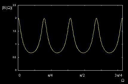
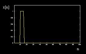
     Filters Examples: Comb Filter 梳状滤波器

        Comb Filter Input            Comb Filter Output

               Input (“Hello?                   Output (“Hello hello?

 

 

 

 

 

 

 

 

 

 

 

 

 

 

 

 

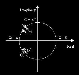
Poles, Zeros & Filter’s Shape

       Single Pole Filter:

    ， ，

            

 

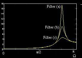
       Three 2-Pole Filters

          

 

         Any Filter:

                  

                 

 

Distance	Filter
Poles Closer to    or Zeros Farther from ejΩ	Larger Gain     More Selective
Poles Farther from or Zeros Closer to  ejΩ	Smaller Gain     Less Selective

           Page 267, Example 7.24 25 26